Chapter 10 Tree Models
10.1 Building Tree Models
library("tree")Use tree() function from library("tree").
tree_fit = tree(y ~ x, data_surrogate)
summary(tree_fit)
##
## Regression tree:
## tree(formula = y ~ x, data = data_surrogate)
## Number of terminal nodes: 3
## Residual mean deviance: 1.001 = 897.9 / 897
## Distribution of residuals:
## Min. 1st Qu. Median Mean 3rd Qu. Max.
## -3.137000 -0.662000 -0.001074 0.000000 0.638100 2.984000#tree_fitsummary(tree_fit) includes a lot of useful information such as the number of terminal nodes and the training misclassification error rate.
Plotting Trees
If pretty = 0 then the level names of a factor split attributes are used unchanged.
plot(tree_fit)
text(tree_fit, pretty=0)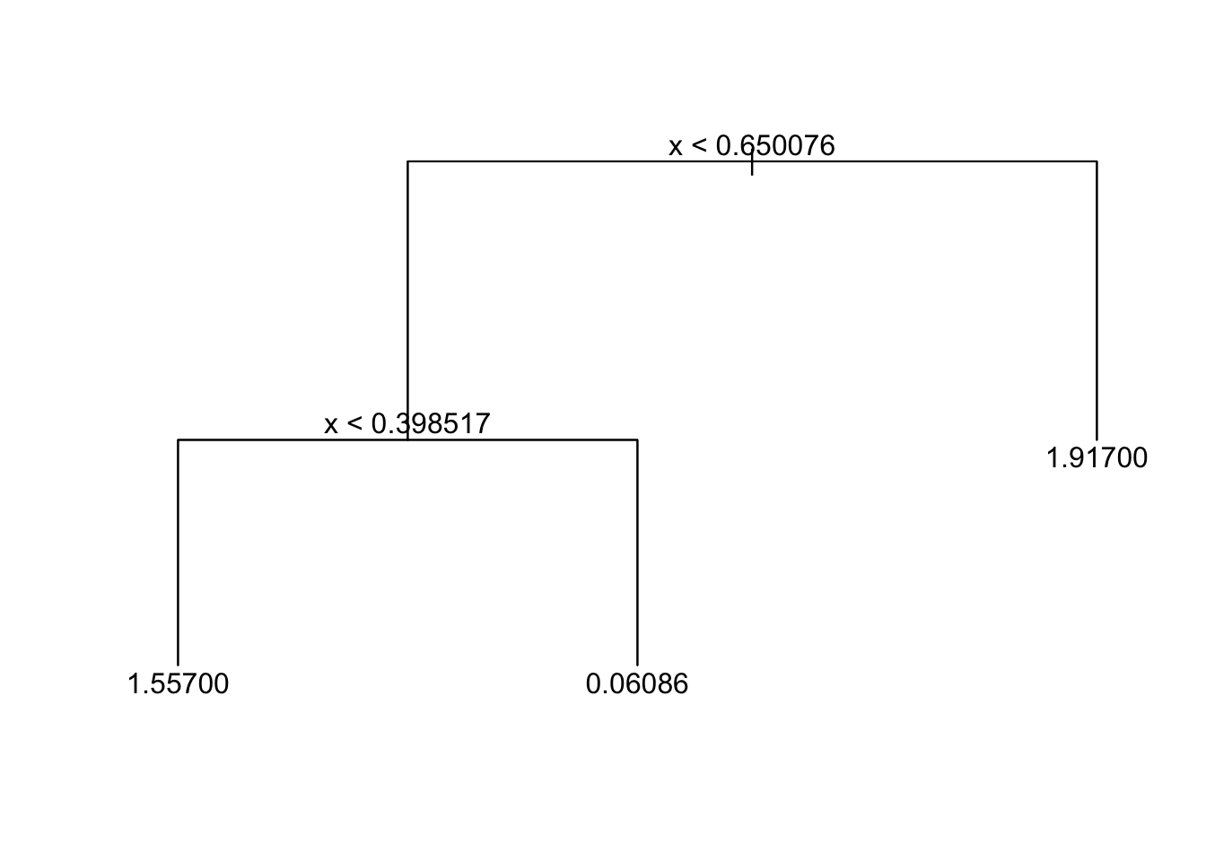
Predictions
Example from practical demonstration with synthetic surrogate data.
set.seed(347)
data_surrogate_test <- data.frame(x = c(runif(200, 0, 0.4), runif(400, 0.4, 0.65), runif(300, 0.65, 1)),
                                  y = c(rnorm(200, 1.5),    rnorm(400, 0),         rnorm(300, 2)))
Use predict() function. The tree model gives the mean in that terminal node group as a prediction.
tree_pred = predict(tree_fit, data_surrogate_test)When you are predicting a factor variable, use type = "class" to specify a prediction from the class.
Plotting Predictions
plot(x = data_surrogate_test$x[1:200], y = data_surrogate_test$y[1:200],
     col = 'blue', xlab = "X", ylab = "Y", pch = 19, xlim = c(0,1), ylim = c(-2,4))
points(x = data_surrogate_test$x[201:600], y = data_surrogate_test$y[201:600], col = 'red', pch = 19)
points(x = data_surrogate_test$x[601:900], y = data_surrogate_test$y[601:900], col = 'green', pch = 19)

points(x=data_surrogate_test$x,y=tree_pred,col='black',pch=15)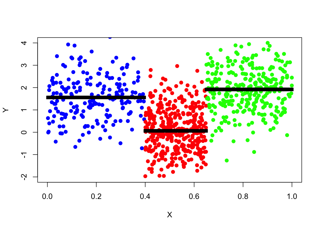
MSE
pred_mse=mean((data_surrogate_test$y-tree_pred)^2)
pred_mse
## [1] 1.005645Calculating Prediction Classification Error (Classification Trees)
Example from mock practical exam:
tree.carseats = tree(High ~ .-Sales, data_train)

tree.pred = predict(tree.carseats, data_test, type="class")
table(tree.pred, data_test$High)
##
## tree.pred No Yes
## No 80 27
## Yes 12 31(80+31)/150## [1] 0.74The percentage of correct predictions is 74%.
Pruning Trees
Prune tree with prune.tree() command, but can first plot the deviance for different size trees using cv.tree() with parameter FUN = prune.tree. Alternatively, can use parameter FUN = prune.misclass to plot misclass (when a classification tree - factor variable).
tree_cv_prune = cv.tree(tree_fit_s, FUN = prune.tree)
#tree_cv_prune
plot(tree_cv_prune)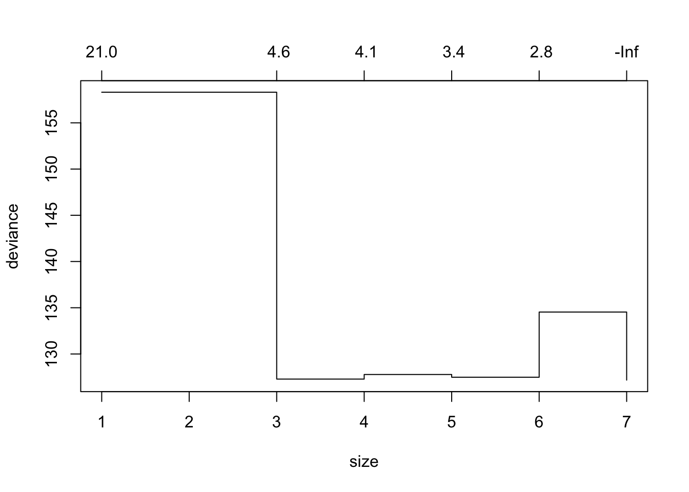
The “best” sized tree (via CV) is the one with the lowest deviance/misclass.
Fitting Pruned Model
tree_fit_prune = prune.tree(tree_fit_s, best = 3)
tree_fit_prune
## node), split, n, deviance, yval
## * denotes terminal node
##
## 1) root 90 131.60 1.0660
## 2) x < 0.653469 60 90.67 0.7376
## 4) x < 0.427732 26 29.65 1.4510 *
## 5) x > 0.427732 34 37.64 0.1917 *
## 3) x > 0.653469 30 21.48 1.7240 *You may also prune the tree by specifying the cost-complexity parameter k, for example tree_fit_prune=prune.tree(tree_fit_s, k=5).
Note for classification trees: Regression trees must use the default method = deviance parameter but for classification trees, this parameter can be deviance or misclass (misclass prefers trees with lower misclassification rate). Shorthand for including method = misclass is to use the prune.misclass function instead of prune.tree.
Pruned Tree:
plot(tree_fit_prune)
text(tree_fit_prune,pretty=0)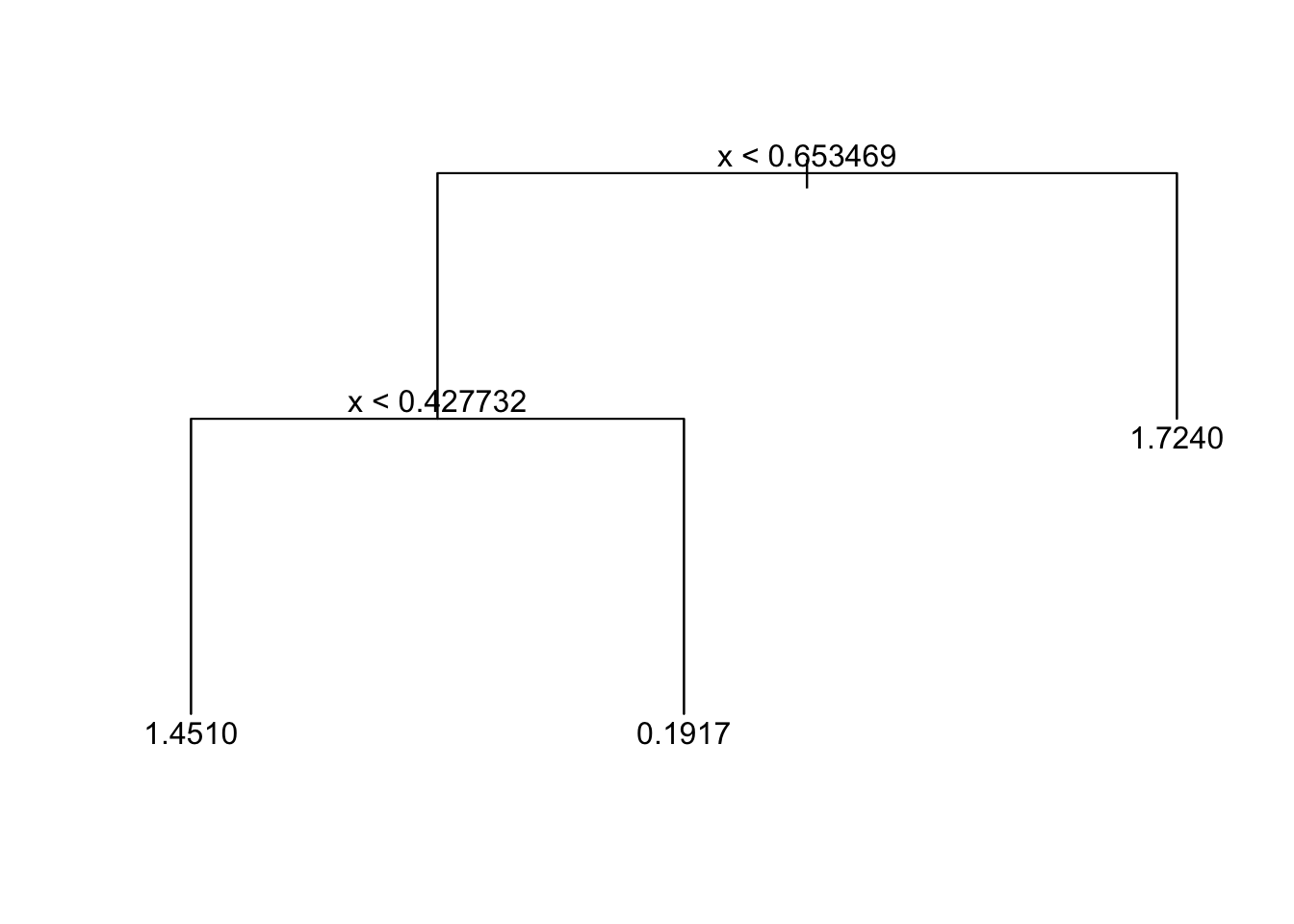
Pruning has decreased the MSE:
tree_pred_prune=predict(tree_fit_prune,data_surrogate_test)
pred_mse_prune = mean((data_surrogate_test$y-tree_pred_prune)^2)
pred_mse - pred_mse_prune
## [1] 0.1765653The following function shows this is a general result and holds on average:
prune_improvement <- function(k) {
  data_surrogate_s <- data.frame(x = c(runif(20, 0, 0.4), runif(40, 0.4, 0.65), runif(30, 0.65, 1)),
                                 y = c(rnorm(20, 1.5),    rnorm(40, 0),         rnorm(30, 2)))
  tree_fit_s = tree(y~x,data_surrogate_s)
  tree_pred_s = predict(tree_fit_s,data_surrogate_test)
  pred_mse_s = mean((data_surrogate_test$y-tree_pred_s)^2)
  tree_fit_prune = prune.tree(tree_fit_s,k=5)
  tree_pred_prune = predict(tree_fit_prune,data_surrogate_test)
  pred_mse_prune = mean((data_surrogate_test$y-tree_pred_prune)^2)
  dif_t = pred_mse_s-pred_mse_prune
  return(dif_t)
}
mean(sapply(1:1024, FUN=function(i){prune_improvement(5)}))
## [1] 0.0992611710.2 Bagging and Random Forests
Follows an example which uses library(ISLR) and library(MASS) for bagging, random forests and boosted trees. We have data_train and data_test from the Boston dataset.
Tree Model and Pruned Tree Model Trained:
tree.boston = tree(medv ~ ., data_train)
prune.boston = prune.tree(tree.boston, best = 6)
Bagging Model
For bagging, we use the library(randomForest) package but with mrty = 13 (\(m = p\) so using all predictors).
Bagging Model (10 Trees):
set.seed (472)
bag.boston = randomForest(medv ~ ., data = data_train, mtry=13, ntree=10, importance = TRUE)
Prediction Accuracy:
pred.bag = predict(bag.boston, newdata = data_test)
plot(pred.bag, data_test$medv, bty = 'l')
abline(0,1)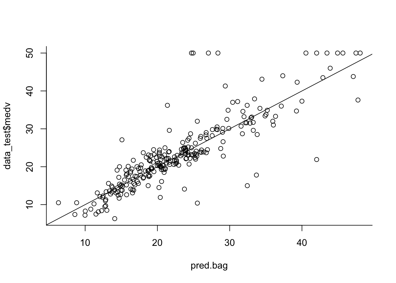
MSE:
mean((pred.bag - data_test$medv)^2)## [1] 23.98799Same for 100 and 1000 trees:
#100 trees
bag.boston = randomForest(medv ~ ., data = data_train, mtry = 13, ntree = 100, importance = TRUE)
pred.bag = predict(bag.boston, newdata = data_test)
mean((pred.bag - data_test$medv)^2) #MSE
## [1] 24.04128#1000 trees
bag.boston = randomForest(medv ~ ., data = data_train, mtry = 13, ntree = 1000, importance = TRUE)
pred.bag = predict(bag.boston, newdata = data_test)
mean((pred.bag - data_test$medv)^2) #MSE## [1] 23.46335Random Forests
Use mtry as something else for random forests. By default this will be \(p/3\) but can also try \(\sqrt{p}\). Very similar method to bagging.
rf.boston = randomForest(medv ~ ., data = data_train, mtry = 4, ntree = 100, importance = TRUE) #uses 4 variables
pred.rf = predict(rf.boston, newdata = data_test)
mean((pred.rf -data_test$medv)^2) #MSE
## [1] 19.23722Importance Plot
importance(rf.boston)## %IncMSE IncNodePurity
## crim 5.141187 1206.45846
## zn 1.862903 216.91995
## indus 3.527213 657.55620
## chas 1.109467 43.61585
## nox 5.448503 1105.66023
## rm 15.393403 6888.75872
## age 5.439751 735.33618
## dis 5.249046 855.71969
## rad 2.117459 163.24660
## tax 4.123422 684.25752
## ptratio 2.589235 963.42017
## black 4.557716 370.96316
## lstat 10.676720 5155.26867?importance
varImpPlot(rf.boston)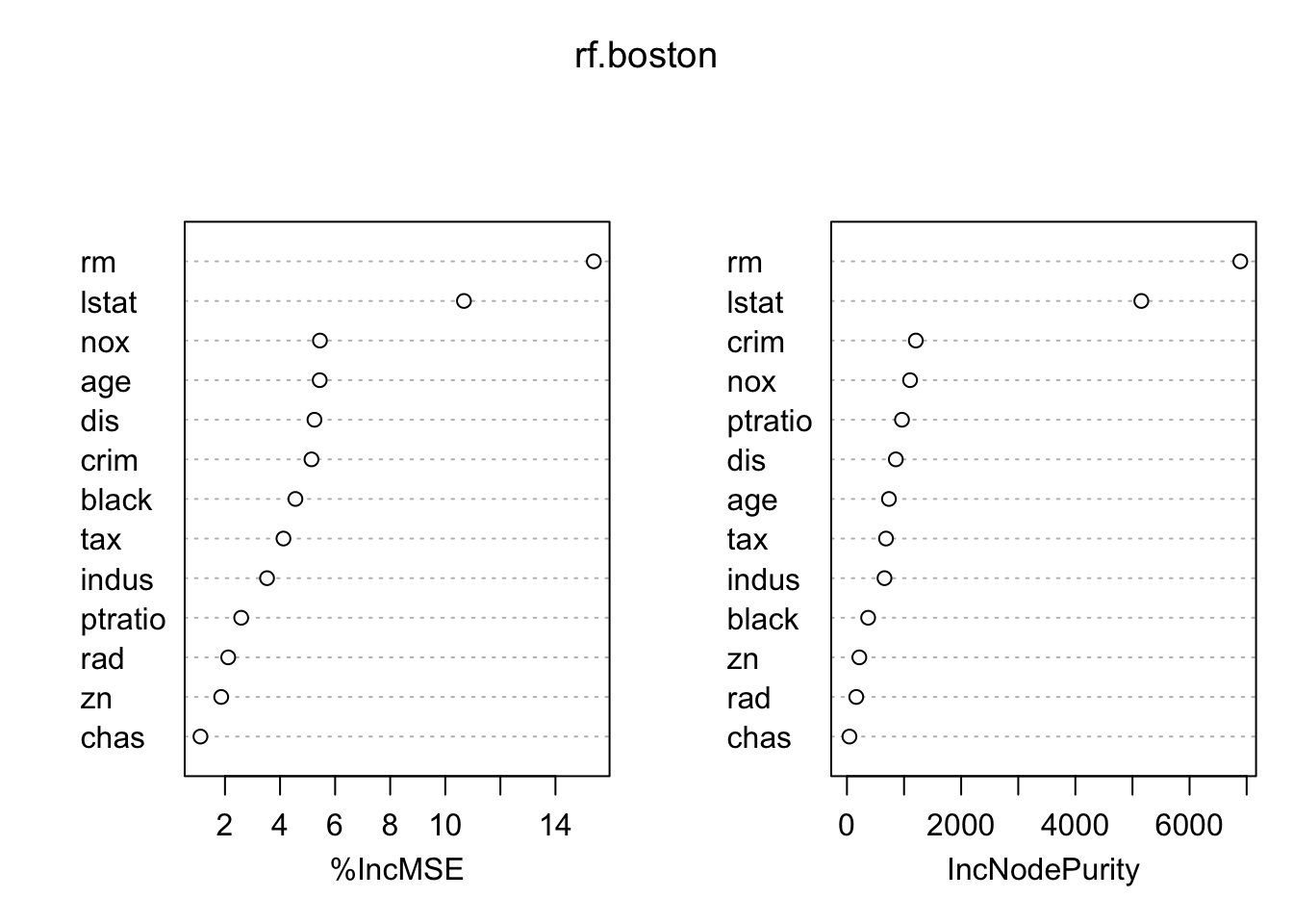
Higher up variables have higher importance (prediction power). MSE and Gini Index usually give similar plots but can differ significantly when there are categorical variables, especially with many levels.
Plotting test error (MSE) for all different mtry()
test.err = double(13) #sequence of all zeros length 13

for(mtry_t in 1:13){
  fit = randomForest(medv ~ ., data = data_train, mtry = mtry_t, ntree = 100)
  pred = predict(fit, data_test)
  test.err[mtry_t] = mean((pred - data_test$medv)^2)
}

plot(test.err, pch = 20)
lines(test.err)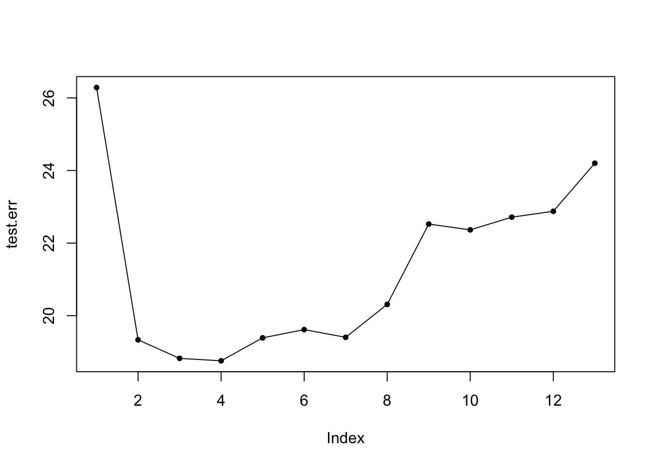
10.3 Boosting
Use the Generalized Boosted Regression Modelling (GBM) Package library(gbm).
library(gbm)For boosted regression trees, use distribution = "gaussian" but for binary classification problems, use distribution = “bernoulli”.
set.seed(517)
boost.boston = gbm(medv ~ ., data = data_train, distribution="gaussian", n.trees = 1000, interaction.depth = 2)
#interaction depth is d in lecture notes
summary(boost.boston) #makes a plot too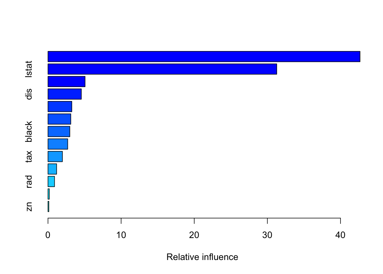
##             var    rel.inf
## rm           rm 42.6691313
## lstat     lstat 31.2820748
## crim       crim  5.0703499
## dis         dis  4.5616872
## nox         nox  3.2604137
## age         age  3.1196043
## black     black  2.9887370
## ptratio ptratio  2.6983302
## tax         tax  1.9729225
## indus     indus  1.1820825
## rad         rad  0.8957232
## chas       chas  0.1816023
## zn           zn  0.1173412
pred.boost = predict(boost.boston, newdata = data_test, n.trees = 1000)
mean((pred.boost-data_test$medv)^2) #MSE - improvement on random forests## [1] 16.98637Interaction depth is the number of splits performed on each tree in the boosting model.
If you want to predict a binary classification problem, use type = "response" in predict() function. The type = "response" option tells R to output probabilities of the form P(Y=1|X) instead of other information such as logit.
Mock Practical Exam Example
library(modeldata)
library(randomForest)
library(gbm)
data(credit_data)
credit_data=na.omit(credit_data)

set.seed(180)
train = sample (1: nrow(credit_data), floor(nrow(credit_data )/2))
data_train=credit_data[train,]
data_test=credit_data[-train,]

boost.credit=gbm(unclass(Status)-1~.,data=data_train,distribution="bernoulli",
                 n.trees =1000,interaction.depth=2)
summary(boost.credit)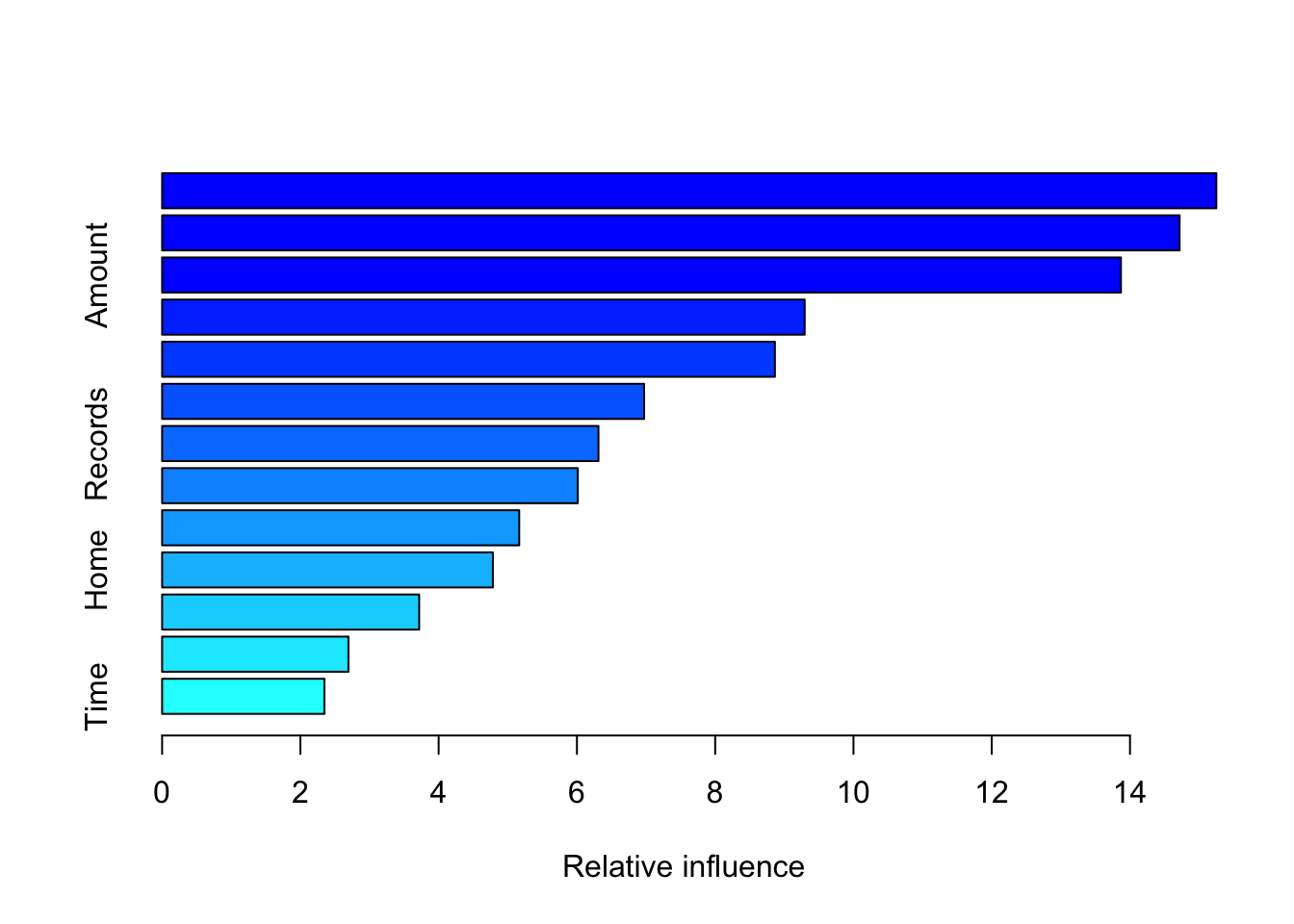
##                 var   rel.inf
## Income       Income 15.249172
## Price         Price 14.717764
## Amount       Amount 13.868971
## Seniority Seniority  9.294412
## Age             Age  8.863564
## Job             Job  6.972005
## Records     Records  6.311414
## Expenses   Expenses  6.012140
## Assets       Assets  5.165404
## Home           Home  4.784225
## Debt           Debt  3.718170
## Marital     Marital  2.695232
## Time Time 2.347527pred.boost=predict(boost.credit,newdata =data_test, n.trees =1000, type="response")
pred.boost.wrong=predict(boost.credit,newdata =data_test, n.trees =1000)
status_pred=ifelse(pred.boost<=0.5,"bad","good")
class_table=table(status_pred, data_test$Status)
success_rate=(class_table[1,1]+class_table[2,2])/sum(class_table)
success_rate## [1] 0.7955446