Chapter 6 Polynomial Regression
Simplest example of a non-linear model.
6.1 Polynomial Regression Model Example (Degree 2)
Following practical demonstration 8.3 we build a model for Boston dataset in library(MASS) which has no missing data. To just see an example see Polynomial Regression (Higher Degrees).
##
## Attaching package: 'MASS'
## The following object is masked from 'package:dplyr':
##
## selectFor convenience, we can rename the response and predictor variable y and x respectively, and label axes for plotting. Below is then a basic plot of response against predictor.
y = Boston$medv
x = Boston$lstat
y.lab = 'Median Property Value'
x.lab = 'Lower Status (%)'plot( x, y, cex.lab = 1.1, col="darkgrey", xlab = x.lab, ylab = y.lab,
main = "", bty = 'l' )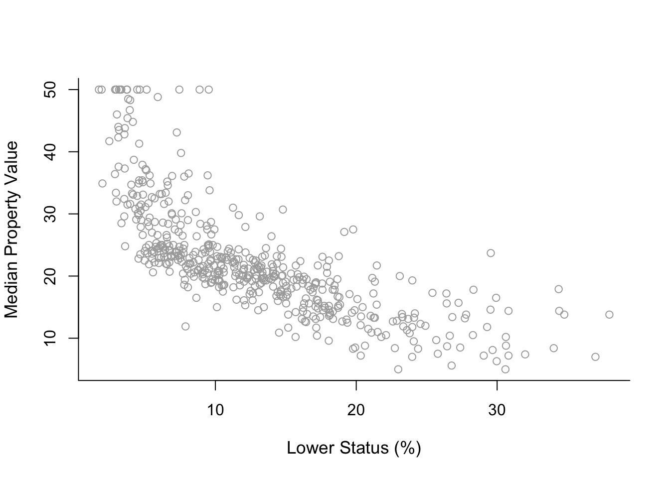
Polynomial Regression Function
Polynomial regression can be called by writing out the predictors directly (poly2 = lm( y ~ x + I(x^2) )), or using the poly() command.
poly2 = lm(y ~ poly(x,  2,  raw = TRUE)) #2 is the degree
#summary(poly2)
Here, raw = TRUE calculates the polynomial regression as usual. Leaving this out so default is raw = FALSE would lead to an orthogonal basis being chosen to perform the regression on.
Plotting Simple Polynomial Regression
First, we mus sort the \(x\) values for the plot to work. We use each initial \(x\) data point as a point we connect between to draw the polynomial.
sort.x = sort(x)
pred2 = predict(poly2, newdata = list(x = sort.x), se = TRUE)
names(pred2)
## [1] "fit" "se.fit" "df" "residual.scale"pred2 contains fit which are the fitted values and se.fit which are the standard errors at each fitted point.
se.bands2 = cbind( pred2$fit - 2 * pred2$se.fit,
                   pred2$fit + 2 * pred2$se.fit )
Final Plot
plot(x, y, cex.lab = 1.1, col="darkgrey", xlab = x.lab, ylab = y.lab,
     main = "Degree-2 polynomial", bty = 'l')
lines(sort.x, pred2$fit, lwd = 2, col = "red")
matlines(sort.x, se.bands2, lwd = 1.4, col = "red", lty = 3)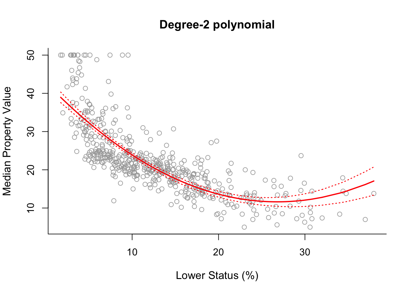
6.2 Polynomial Regression (Higher Degrees)
poly3 = lm(y ~ poly(x,  3))
poly4 = lm(y ~ poly(x,  4))
poly5 = lm(y ~ poly(x, 5))

pred3 = predict(poly3, newdata = list(x = sort.x), se = TRUE)
pred4 = predict(poly4, newdata = list(x = sort.x), se = TRUE)
pred5 = predict(poly5, newdata = list(x = sort.x), se = TRUE)

se.bands3 = cbind(pred3$fit + 2*pred3$se.fit, pred3$fit-2*pred3$se.fit)
se.bands4 = cbind(pred4$fit + 2*pred4$se.fit, pred4$fit-2*pred4$se.fit)
se.bands5 = cbind(pred5$fit + 2*pred5$se.fit, pred5$fit-2*pred5$se.fit)


par(mfrow = c(2,2))
# Degree-2
plot(x, y, cex.lab = 1.1, col="darkgrey", xlab = x.lab, ylab = y.lab,
     main = "Degree-2 polynomial", bty = 'l')
lines(sort.x, pred2$fit, lwd = 2, col = "red")
matlines(sort.x, se.bands2, lwd = 2, col = "red", lty = 3)

# Degree-3
plot(x, y, cex.lab = 1.1, col="darkgrey", xlab = x.lab, ylab = y.lab,
     main = "Degree-3 polynomial", bty = 'l')
lines(sort.x, pred3$fit, lwd = 2, col = "darkviolet")
matlines(sort.x, se.bands3, lwd = 2, col = "darkviolet", lty = 3)

# Degree-4
plot(x, y, cex.lab = 1.1, col="darkgrey", xlab = x.lab, ylab = y.lab,
     main = "Degree-4 polynomial", bty = 'l')
lines(sort.x, pred4$fit, lwd = 2, col = "blue")
matlines(sort.x, se.bands4, lwd = 2, col = "blue", lty = 3)

# Degree-5
plot(x, y, cex.lab = 1.1, col="darkgrey", xlab = x.lab, ylab = y.lab,
     main = "Degree-5 polynomial", bty = 'l')
lines(sort.x, pred5$fit, lwd = 2, col = "black")
matlines(sort.x, se.bands5, lwd = 2, col = "black", lty = 3)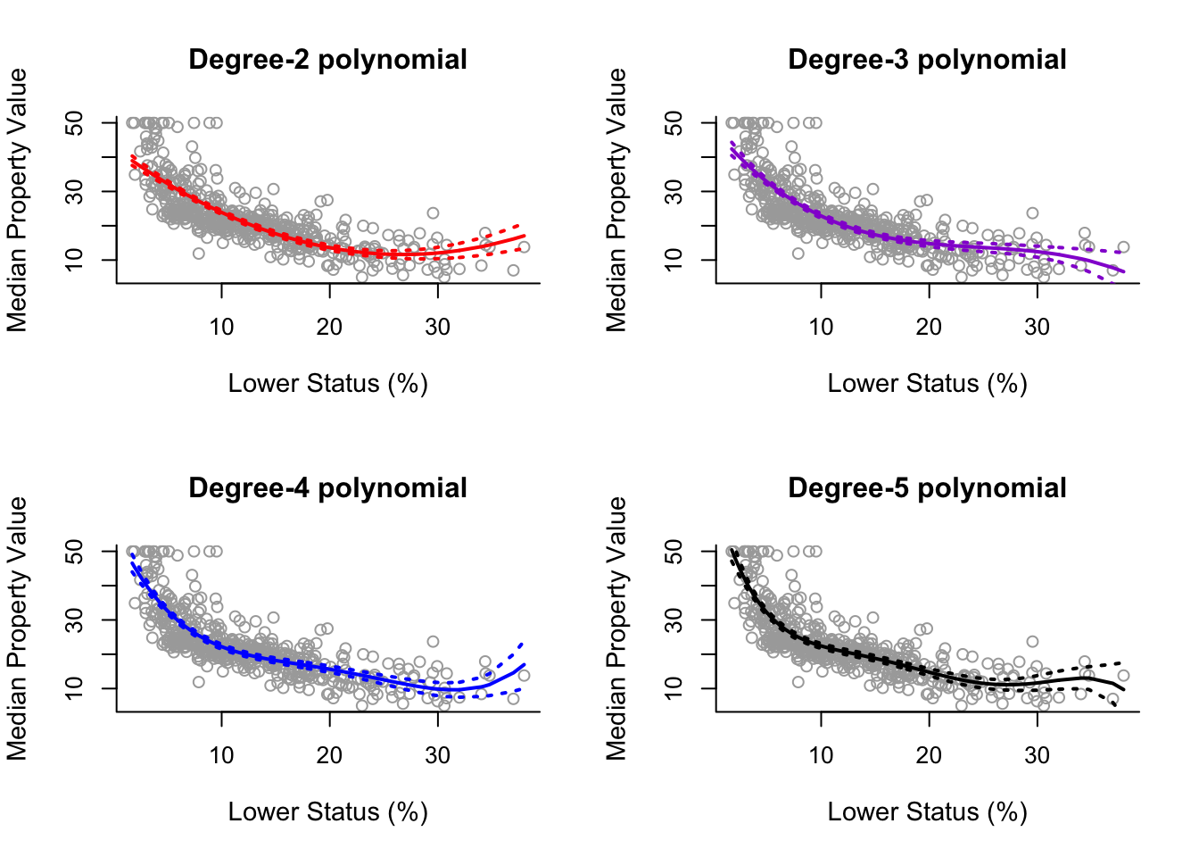
6.3 Choosing a Degree (ANOVA)
This can be done by F-test comparison (analysis of variance - ANOVA) or Cross-Validation. With all the polynomial models trained, we can compare them with the function anova().
anova(poly1, poly2, poly3, poly4, poly5, poly6)## Analysis of Variance Table
##
## Model 1: y ~ x
## Model 2: y ~ poly(x, 2, raw = TRUE)
## Model 3: y ~ poly(x, 3)
## Model 4: y ~ poly(x, 4)
## Model 5: y ~ poly(x, 5)
## Model 6: y ~ poly(x, 6)
## Res.Df RSS Df Sum of Sq F Pr(>F)
## 1 504 19472
## 2 503 15347 1 4125.1 151.8623 < 2.2e-16 ***
## 3 502 14616 1 731.8 26.9390 3.061e-07 ***
## 4 501 13968 1 647.8 23.8477 1.406e-06 ***
## 5 500 13597 1 370.7 13.6453 0.0002452 ***
## 6 499 13555 1 42.4 1.5596 0.2123125
## ---
## Signif. codes: 0 '***' 0.001 '**' 0.01 '*' 0.05 '.' 0.1 ' ' 1Looking at the column Pr(>F), reading down the column, if it is less than a significance level (say 0.05) then accept adding a higher degree and if it isn’t stop on whatever degree model you have. So we would end up with a degree 5 polynomial model in this example.