Chapter 5 Shrinkage Methods

5.1 Ridge and Lasso Regression

Performing Ridge Regression

To perform ridge regression, we use the package glmnet.

library(glmnet)

Important Note: glmnet() uses different syntax than regsubsets().

Continuing example with Hitters data,

y = Hitters$Salary
# Here we exclude the first column because it corresponds to the intercept.
x = model.matrix(Salary ~ ., Hitters)[,-1]

Note that model.matrix(Salary ~ ., Hitters)[,-1] is exactly the same as Hitters[,-19] (Salary has index 19), it just is all the data for the prediction variables.

Performing ridge regression just involves using the glmnet() function specifying alpha = 0 (for ridge).

ridge = glmnet(x, y, alpha = 0)

To use a different number of $\lambda$, change parameter nlambda which is 100 by default.

Extracting Information

names(ridge)

##  [1] "a0"        "beta"      "df"        "dim"       "lambda"    "dev.ratio"
##  [7] "nulldev"   "npasses"   "jerr"      "offset"    "call"      "nobs"

ridge$beta contains the values of the coefficients under each $\lambda$ (use ridge$beta[,1:3] to see first 3 for example).
coef(ridge) contains exact same information as ridge$beta but also includes intercept estimates.
ridge$lambda contains the grid of all $\lambda$ values that were used.

5.1.1 Performing Lasso regression

Very similar to ridge but with alpha = 1 in glmnet(), which is the default so doesn’t need to be specified.

y = Hitters$Salary
x = model.matrix(Salary~., Hitters)[,-1]

lasso = glmnet(x, y)

Plotting Regularisation Paths

xvar = 'lambda' specifies to plot coefficient values against Log $\lambda$, otherwise the default xvar is the $L_1$ Norm. Below are two examples, it is the exact same method for ridge and lasso

Ridge Coefficients Against Log $\lambda$

plot(ridge, xvar = 'lambda')

Lasso Coefficients Against $L_1$ Norm

plot(lasso)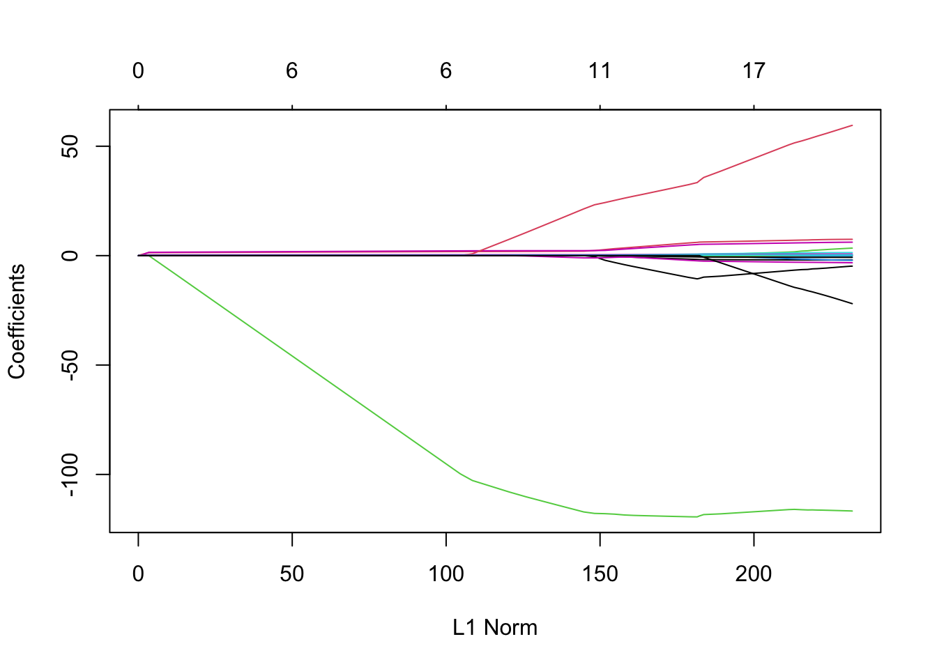

Cross-Validation

To find best $\lambda$ with cross-validation, use cv.glmnet() instead.

ridge.cv = cv.glmnet(x, y, alpha=0)
names(ridge.cv)

##  [1] "lambda"     "cvm"        "cvsd"       "cvup"       "cvlo"      
##  [6] "nzero"      "call"       "name"       "glmnet.fit" "lambda.min"
## [11] "lambda.1se" "index"

ridge.cv$lambda.min gives the optimal $\lambda$.
ridge.cv$lambda.1se gives the maximum $\lambda$ 1 standard-error away from optimal lambda.

Plotting

In the plot below, the left dotted line highlights value of lambda.min and the right dotted line hightlights value of lambda.1se.

plot(ridge.cv)
abline( h = ridge.cv$cvup[ridge.cv$index[1]], lty = 4 )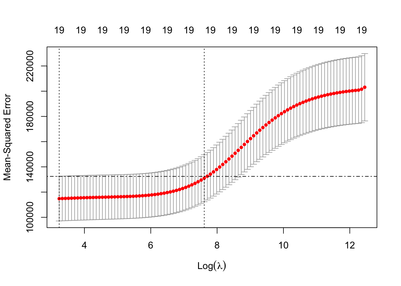

To add these to the plots of coefficients against Log $\lambda$,

plot(ridge, xvar = 'lambda')
abline(v = log(ridge.cv$lambda.min), lty = 3) # careful to use the log here and below
abline(v = log(ridge.cv$lambda.1se), lty = 3)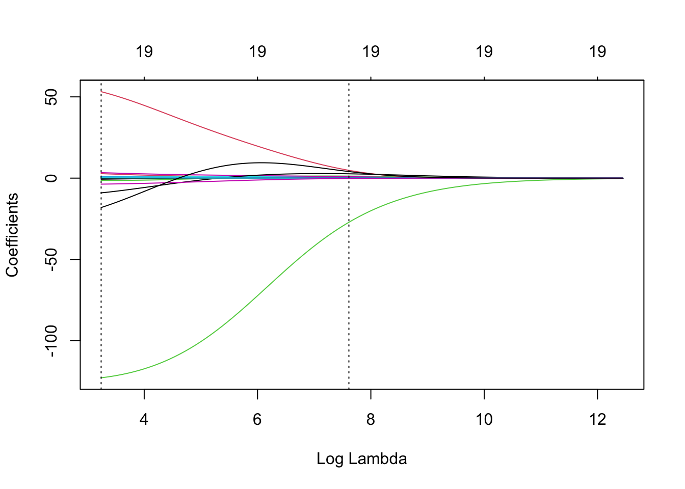

5.1.2 Comparing Predictive Performance For Different $\lambda$s

See another example of this method applied to BSS, Ridge, Lasso and PCR at end of this chapter.

repetitions = 50
mse.1 = c()
mse.2 = c()

set.seed(1)                
for(i in 1:repetitions){
  
  # Step (i) random data splitting
  training.obs = sample(1:263,  175)
  y.train = Hitters$Salary[training.obs]
  x.train = model.matrix(Salary~., Hitters[training.obs, ])[,-1]
  y.test = Hitters$Salary[-training.obs]
  x.test = model.matrix(Salary~., Hitters[-training.obs, ])[,-1]
  
  # Step (ii) training phase
  lasso.train = cv.glmnet(x.train, y.train)
  
  # Step (iii) generating predictions
  predict.1 = predict(lasso.train, x.test, s = 'lambda.min')
  predict.2 = predict(lasso.train, x.test, s = 'lambda.1se')
  
  # Step (iv) evaluating predictive performance
  mse.1[i] = mean((y.test-predict.1)^2)
  mse.2[i] = mean((y.test-predict.2)^2)
}

boxplot(mse.1, mse.2, names = c('min-CV lasso','1-se lasso'), 
        ylab = 'Test MSE', col = 7)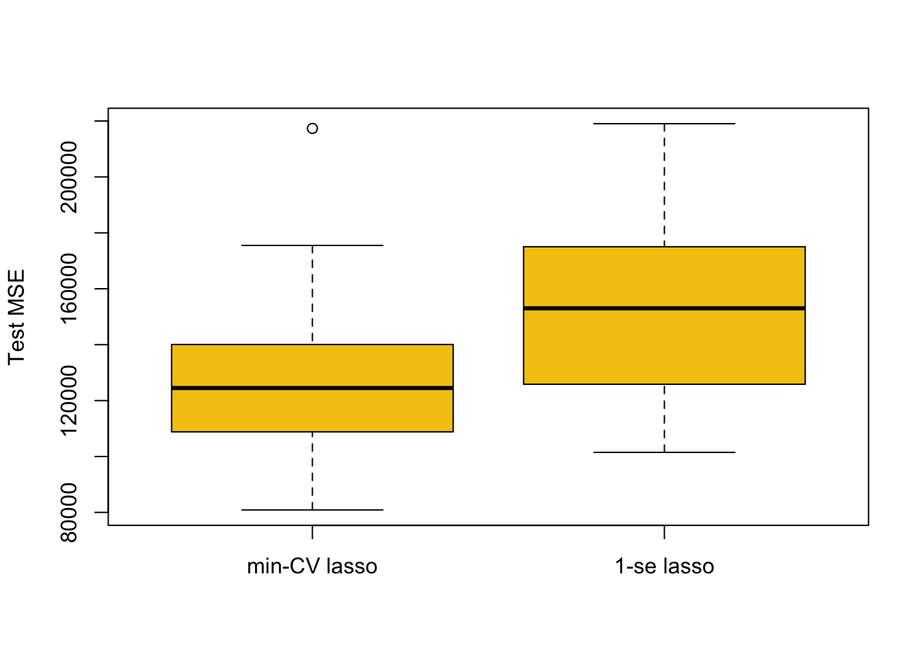

5.2 Principal Component Analysis

This section contains many examples from practical 3. We use seatpos (38x9 dimension and no missing values) data from faraway package.

library(faraway)

To perform principal component analysis without cross-validation, use prcomp() function.

Seperate out response and prediction variables into x and y

y <- seatpos$hipcenter
x <- model.matrix(hipcenter ~ ., seatpos)[,-1]

Note that model.matrix(hipcenter ~ ., seatpos)[,-1] is equivalent to seatpos[,-9].

seatpos.pr <- prcomp(x, scale=TRUE)

Scaling - scale = TRUE scales each variable by it’s standard error which is needed for meaningful inference. However, this can also be done manually, - To manually scale before running prcomp, divide by column standard errors,

s <- apply(x, 2, sd)         # calculates the column SDs
x.s  <- sweep(x, 2, s, "/")  # divides all columns by their SDs

Extracting Data

Variance: seatpos.pr$sdev gives the standard deviation of each component (seatpos.pr$sdev^2 for variance)
Eigenvectors: seatpos.pr$rotation gives the eigenvectors of each component

These two are equivalent to calling ...$values and ...$vectors on eigen(var(seatpos.s)) where seatpos.s is seatpos manually scaled (alternatively, don’t scale when calling prcom()).

Scree Plots and Proportion of Variance Explained

To manually calculate the proportion of variance each PC explains use,

seatpos.pr$sdev^2 / sum(seatpos.pr$sdev^2 )

## [1] 0.7091482088 0.1545982512 0.0579679303 0.0301197935 0.0242774455
## [6] 0.0173967750 0.0062930659 0.0001985298

Or can directly read off the summary (including cumulative proportions),

summary(seatpos.pr)

## Importance of components:
##                           PC1    PC2     PC3     PC4     PC5    PC6     PC7
## Standard deviation     2.3818 1.1121 0.68099 0.49088 0.44070 0.3731 0.22438
## Proportion of Variance 0.7091 0.1546 0.05797 0.03012 0.02428 0.0174 0.00629
## Cumulative Proportion  0.7091 0.8638 0.92171 0.95183 0.97611 0.9935 0.99980
##                            PC8
## Standard deviation     0.03985
## Proportion of Variance 0.00020
## Cumulative Proportion  1.00000

This is the information a Scree Plot shows which can be plotted straight from the call to prcomp(),

plot(seatpos.pr)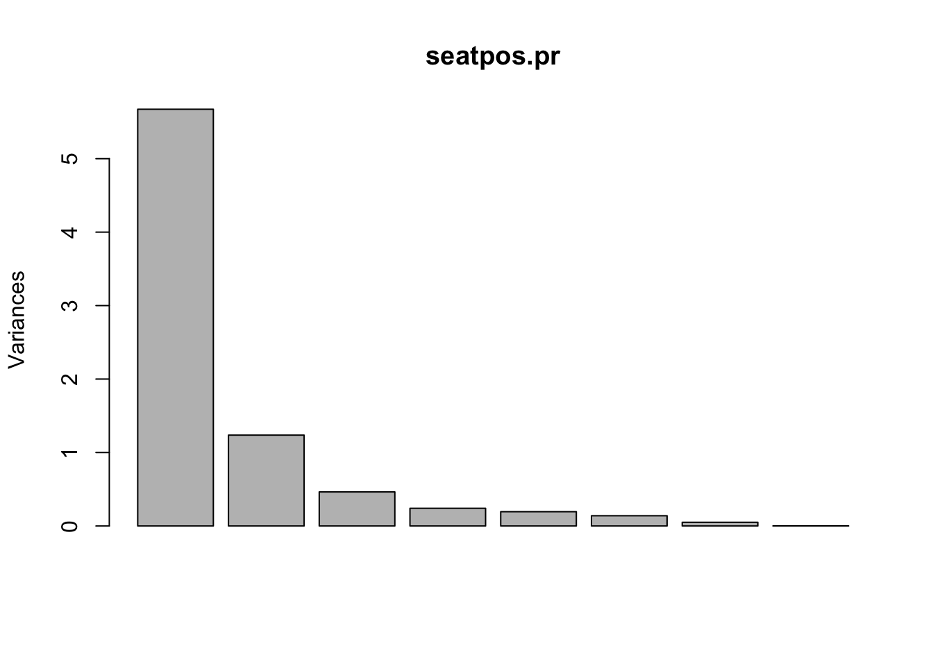

Data Compression (Projection)

Scale data beforehand using manual scaling (see above),

x.s <- sweep(x, 2, apply(x, 2, sd) , "/") #scaled data
seatpos.pr <- prcomp(x.s)

Compress data to $k$ PCs, calculate their means and then reconstruct the data (with error),

T <- t(seatpos.pr$x[,c(1,2,3,4)]) # Compressed using 4 PCs
ms <- colMeans(x.s) # calculates means of scaled data set
R <- t(ms + seatpos.pr$rot[,c(1,2,3,3)]%*% T) # reconstruction

plot(rbind(x.s[,1:2], R[,1:2]), col=c(rep(4,38),rep(2,38)))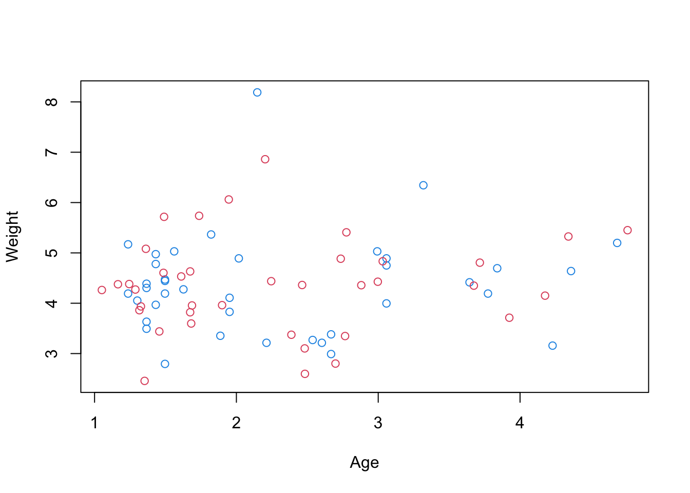

Original data is blue, reconstructions are red

Note: The above only plots two variables, we can plot all pairs using

pairs(rbind(x.s, R), col=c(rep(4,38),rep(2,38)))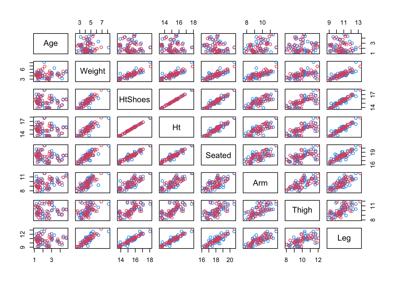

Principal Component Regression

To perform principal component regression we use pls package.

library(pls)

PCR is done with the pcr(function). We continue with Hitters data,

pcr.fit = pcr( Salary ~ ., data = Hitters, scale = TRUE, validation = "CV" )
summary(pcr.fit)

## Data:    X dimension: 263 19 
##  Y dimension: 263 1
## Fit method: svdpc
## Number of components considered: 19
## 
## VALIDATION: RMSEP
## Cross-validated using 10 random segments.
##        (Intercept)  1 comps  2 comps  3 comps  4 comps  5 comps  6 comps
## CV             452    352.5    351.6    352.3    350.7    346.1    345.5
## adjCV          452    352.1    351.2    351.8    350.1    345.5    344.6
##        7 comps  8 comps  9 comps  10 comps  11 comps  12 comps  13 comps
## CV       345.4    348.5    350.4     353.2     354.5     357.5     360.3
## adjCV    344.5    347.5    349.3     351.8     353.0     355.8     358.5
##        14 comps  15 comps  16 comps  17 comps  18 comps  19 comps
## CV        352.4     354.3     345.6     346.7     346.6     349.4
## adjCV     350.2     352.3     343.6     344.5     344.3     346.9
## 
## TRAINING: % variance explained
##         1 comps  2 comps  3 comps  4 comps  5 comps  6 comps  7 comps  8 comps
## X         38.31    60.16    70.84    79.03    84.29    88.63    92.26    94.96
## Salary    40.63    41.58    42.17    43.22    44.90    46.48    46.69    46.75
##         9 comps  10 comps  11 comps  12 comps  13 comps  14 comps  15 comps
## X         96.28     97.26     97.98     98.65     99.15     99.47     99.75
## Salary    46.86     47.76     47.82     47.85     48.10     50.40     50.55
##         16 comps  17 comps  18 comps  19 comps
## X          99.89     99.97     99.99    100.00
## Salary     53.01     53.85     54.61     54.61

Optimal Number of PCs

This is not built in so can be read off from summary above or copy and paste this code,

min.pcr = which.min( MSEP( pcr.fit )$val[1,1, ] ) - 1
min.pcr

## 7 comps 
##       7

MSE Validation Plot

validationplot( pcr.fit, val.type = 'MSEP' )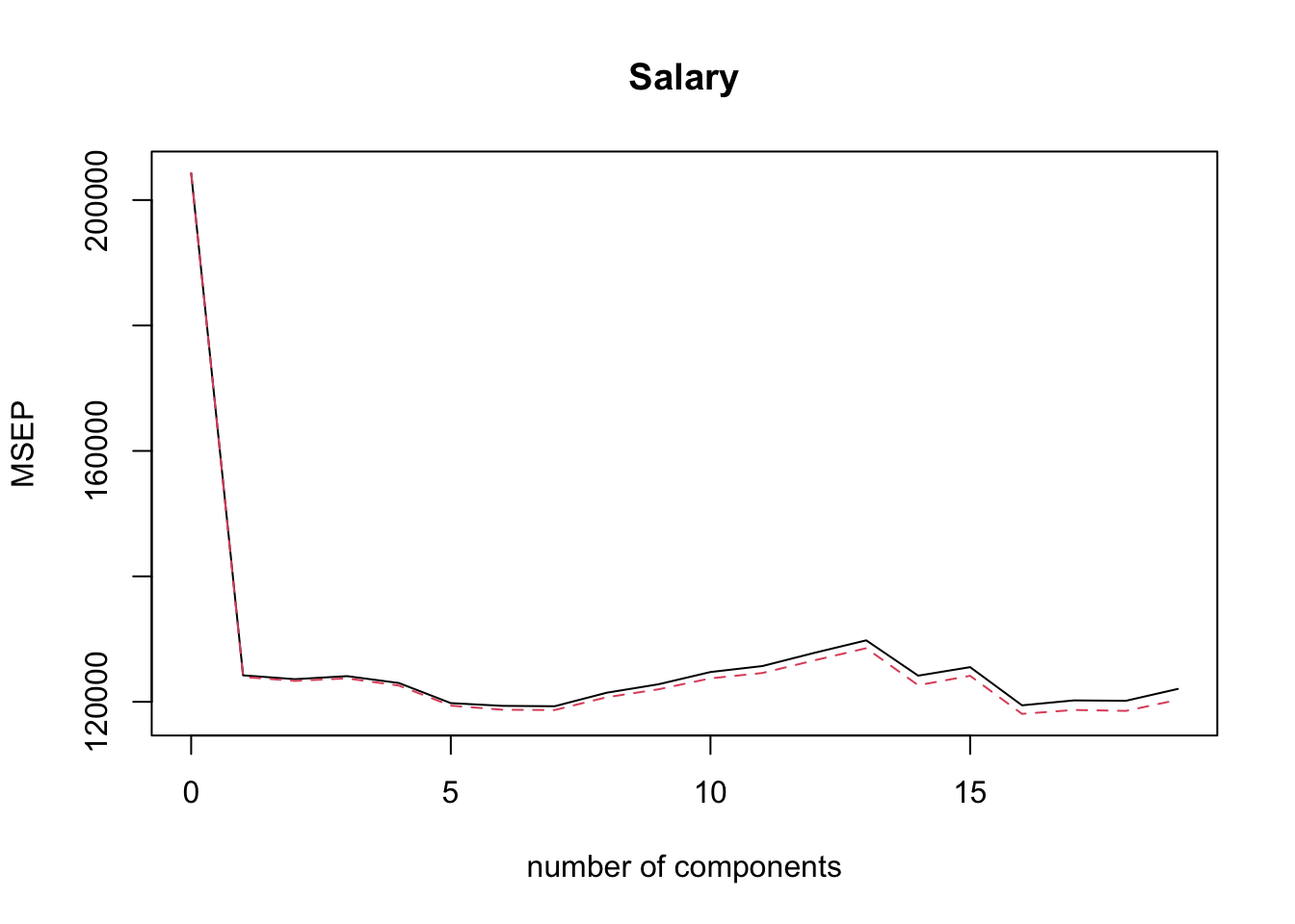

Coefficients of Optimal Number of PCs

coef(pcr.fit, ncomp = min.pcr)

## , , 7 comps
## 
##                Salary
## AtBat       27.005477
## Hits        28.531195
## HmRun        4.031036
## Runs        29.464202
## RBI         18.974255
## Walks       47.658639
## Years       24.125975
## CAtBat      30.831690
## CHits       32.111585
## CHmRun      21.811584
## CRuns       34.054133
## CRBI        28.901388
## CWalks      37.990794
## LeagueN      9.021954
## DivisionW  -66.069150
## PutOuts     74.483241
## Assists     -3.654576
## Errors      -6.004836
## NewLeagueN  11.401041

Similarly, familiar functions like predict can also be used on pcr.fit and has an ncomp parameter.

Regularisation Path Plots

Full explanation of code is at the end of section 7.6.

coef.mat = matrix(NA, 19, 19)
for(i in 1:19){
  coef.mat[,i] = pcr.fit$coefficients[,,i]
}

plot(coef.mat[1,], type = 'l', ylab = 'Coefficients', 
     xlab = 'Number of components', ylim = c(min(coef.mat), max(coef.mat)))
for(i in 2:19){
  lines(coef.mat[i,], col = i)
}

abline(v = min.pcr, lty = 3)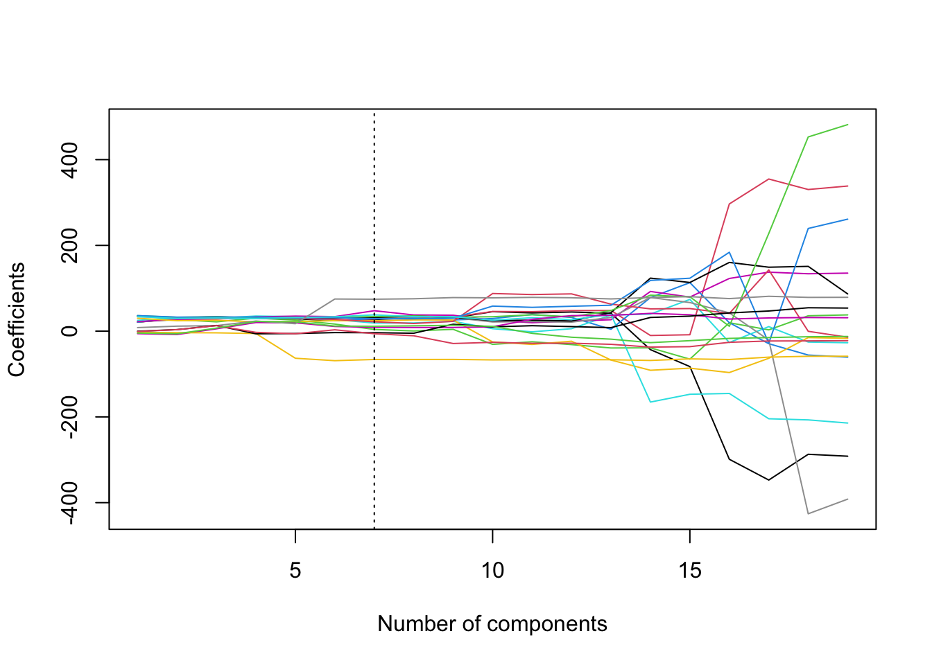

Scree Plots with PCR (manually)

PVE <- rep(NA,19)
for(i in 1:19){ PVE[i]<- sum(pcr.fit$Xvar[1:i])/pcr.fit$Xtotvar }
barplot( PVE, names.arg = 1:19, main = "scree plot", 
         xlab = "number of PCs", 
         ylab = "proportion of variance explained" )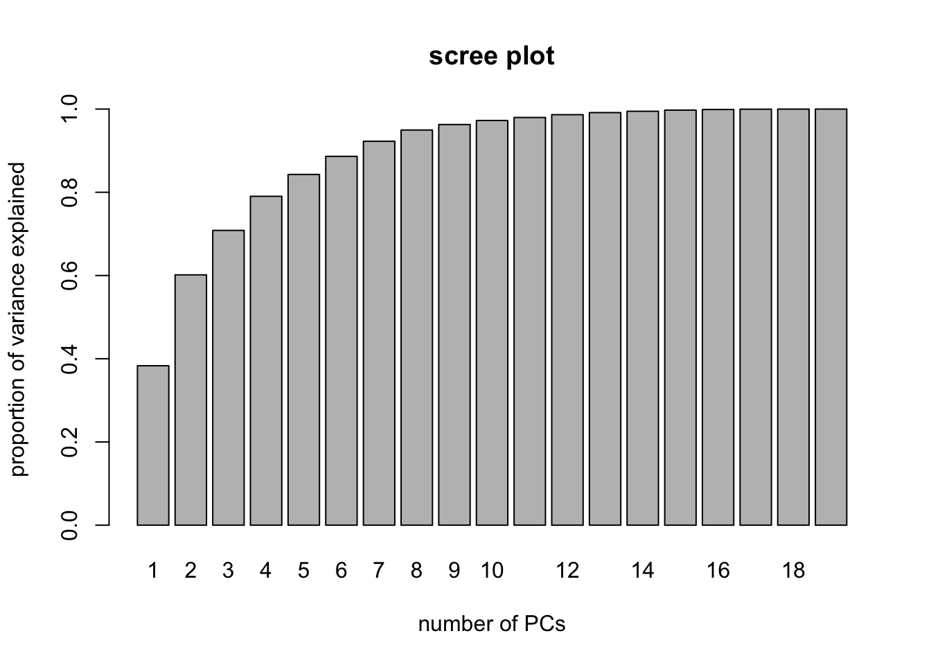

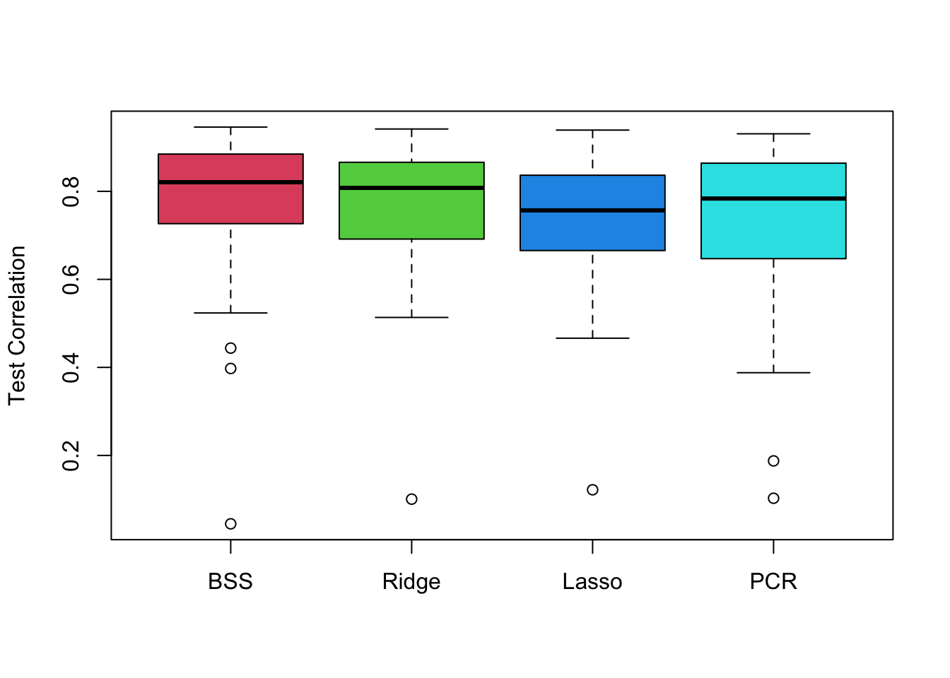
5.3 Comparing Predictive Performances

Example for practical 3. Uses leaps, pls and glmnet packages and we’re give we want to split data training:test as 28:10.

We also need to include predict.regsubsets from chapter 4.

predict.regsubsets = function(object, newdata, id, ...){
  form = as.formula(object$call[[2]])
  mat = model.matrix(form, newdata)
  coefi = coef(object, id = id)
  xvars = names(coefi)
  mat[, xvars]%*%coefi
}

We want to calculate the correlation and MSE for the four models BSS ($C_p$), Ridge (5 folds CV), Lasso (5 fold CV) and PCR over 50 repetitions.

cor.bss = c()
cor.ridge = c()
cor.lasso = c()
cor.pcr = c()
mse.bss = c()
mse.ridge = c()
mse.lasso = c()
mse.pcr = c()

for(i in 1:repetitions){
  # Step (i) data splitting
  training.obs = sample(1:38,  28)
  y.train = seatpos$hipcenter[training.obs]
  x.train = model.matrix(hipcenter ~ ., seatpos[training.obs, ])[,-1]
  y.test = seatpos$hipcenter[-training.obs]
  x.test = model.matrix(hipcenter ~ ., seatpos[-training.obs, ])[,-1]
  
  # Step (ii) training phase
  bss.train = regsubsets(hipcenter ~ ., seatpos, nvmax = 8)
  min.cp = which.min(summary(bss.train)$cp)

  ridge.train = cv.glmnet(x.train, y.train, alpha = 0, nfold=5)
  lasso.train = cv.glmnet(x.train, y.train, nfold=5)
  
  pcr.train = pcr(hipcenter ~ ., data = seatpos[training.obs,],
                  scale = TRUE, validation = "CV" )
  min.pcr = which.min(MSEP(pcr.train)$val[1,1, ] ) - 1
  
  # Step (iii) generating predictions
  predict.bss = predict.regsubsets(bss.train, seatpos[-training.obs, ], min.cp)
  predict.ridge = predict(ridge.train, x.test, s = 'lambda.min')
  predict.lasso = predict(lasso.train, x.test, s = 'lambda.min')
  predict.pcr = predict(pcr.train, seatpos[-training.obs, ], ncomp = min.pcr )
  
  # Step (iv) evaluating predictive performance
  mse.bss[i] = mean((y.test-predict.bss)^2)
  mse.ridge[i] = mean((y.test-predict.ridge)^2)
  mse.lasso[i] = mean((y.test-predict.lasso)^2)
  mse.pcr[i] = mean((y.test-predict.pcr)^2)
  
  cor.bss[i] = cor(y.test, predict.bss)
  cor.ridge[i] = cor(y.test, predict.ridge)
  cor.lasso[i] = cor(y.test, predict.lasso)
  cor.pcr[i] = cor(y.test, predict.pcr)
}

We can then compare with boxplots

boxplot(mse.bss, mse.ridge, mse.lasso, mse.pcr, names = c('BSS','Ridge','Lasso','PCR'), 
        ylab = 'Test MSE', col = 2:5)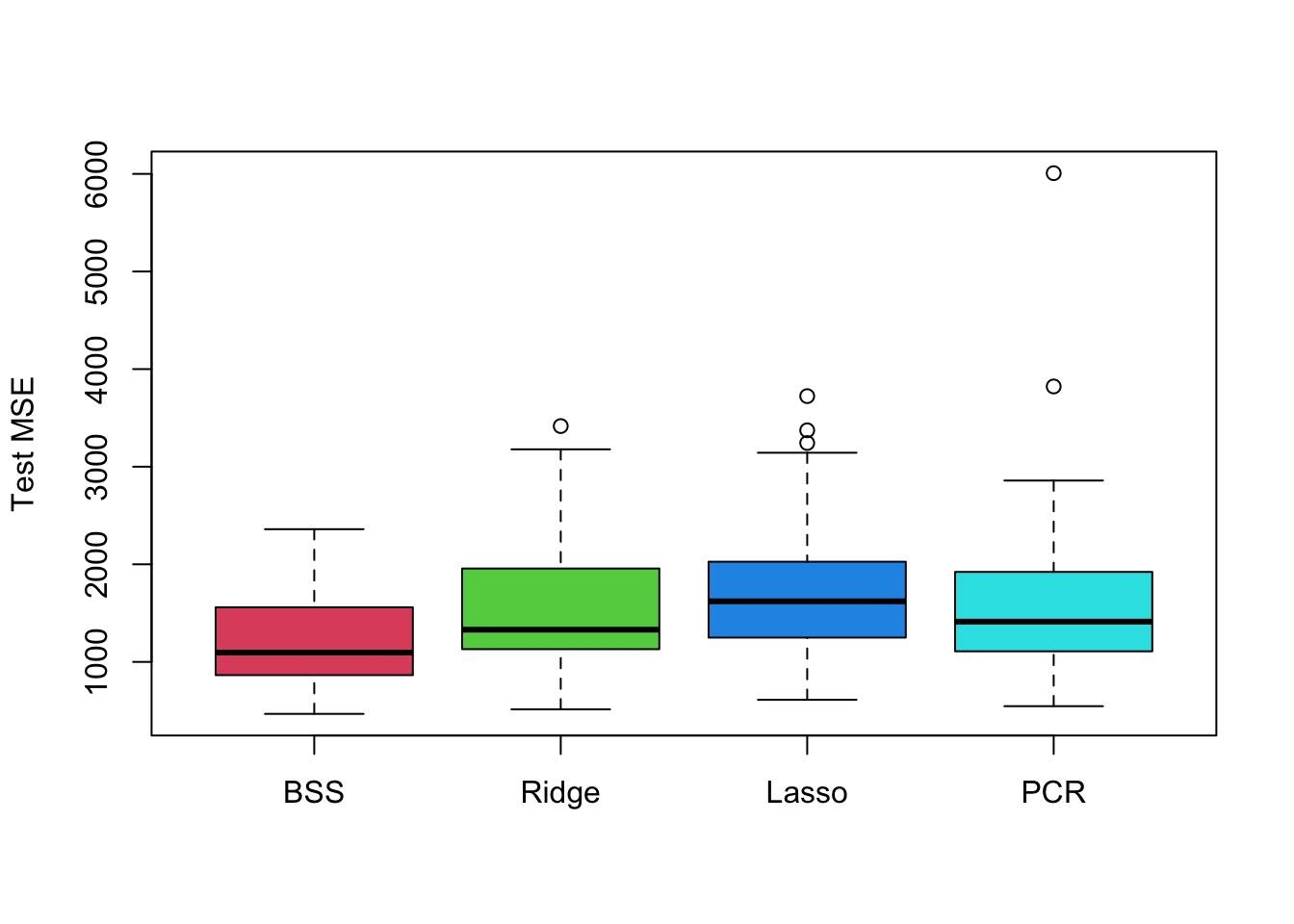

boxplot(cor.bss, cor.ridge, cor.lasso, cor.pcr, names = c('BSS','Ridge','Lasso','PCR'), 
        ylab = 'Test Correlation', col = 2:5)

R Notes