Chapter 9 Logistic Regression

For estimating probability of a qualitative variable. See MLLN Notes for exploratory plots and motivation.

9.1 Simple Logistic Regression

We use the Default data from library("ISLR2") package. We also load library(scales) package for transparency with colours.

## 
## Attaching package: 'scales'

## The following object is masked from 'package:purrr':
## 
##     discard

## The following object is masked from 'package:readr':
## 
##     col_factor

## 
## Attaching package: 'ISLR2'

## The following objects are masked _by_ '.GlobalEnv':
## 
##     Boston, Hitters

## The following object is masked from 'package:MASS':
## 
##     Boston

## The following objects are masked from 'package:ISLR':
## 
##     Auto, Credit

We use the generalised linear model function glm() with family = "binomial".

data(Default)

glm.fit = glm( as.numeric(Default$default=="Yes") ~ balance, data = Default, family = "binomial")
summary(glm.fit)

## 
## Call:
## glm(formula = as.numeric(Default$default == "Yes") ~ balance, 
##     family = "binomial", data = Default)
## 
## Deviance Residuals: 
##     Min       1Q   Median       3Q      Max  
## -2.2697  -0.1465  -0.0589  -0.0221   3.7589  
## 
## Coefficients:
##               Estimate Std. Error z value Pr(>|z|)    
## (Intercept) -1.065e+01  3.612e-01  -29.49   <2e-16 ***
## balance      5.499e-03  2.204e-04   24.95   <2e-16 ***
## ---
## Signif. codes:  0 '***' 0.001 '**' 0.01 '*' 0.05 '.' 0.1 ' ' 1
## 
## (Dispersion parameter for binomial family taken to be 1)
## 
##     Null deviance: 2920.6  on 9999  degrees of freedom
## Residual deviance: 1596.5  on 9998  degrees of freedom
## AIC: 1600.5
## 
## Number of Fisher Scoring iterations: 8

summary(glm.fit$fitted.values)

##      Min.   1st Qu.    Median      Mean   3rd Qu.      Max. 
## 0.0000237 0.0003346 0.0021888 0.0333000 0.0142324 0.9810081

Plot

#Raw Data 
plot(Default$balance, as.numeric(Default$default=="Yes"),col="red",xlab="balance",ylab="default")

#Fitted Values
points(glm.fit$data$balance,glm.fit$fitted.values, col = "black", pch = 4)

#Model Curve
curve(predict(glm.fit,data.frame(balance = x),type="resp"),col="blue",lwd=2,add=TRUE)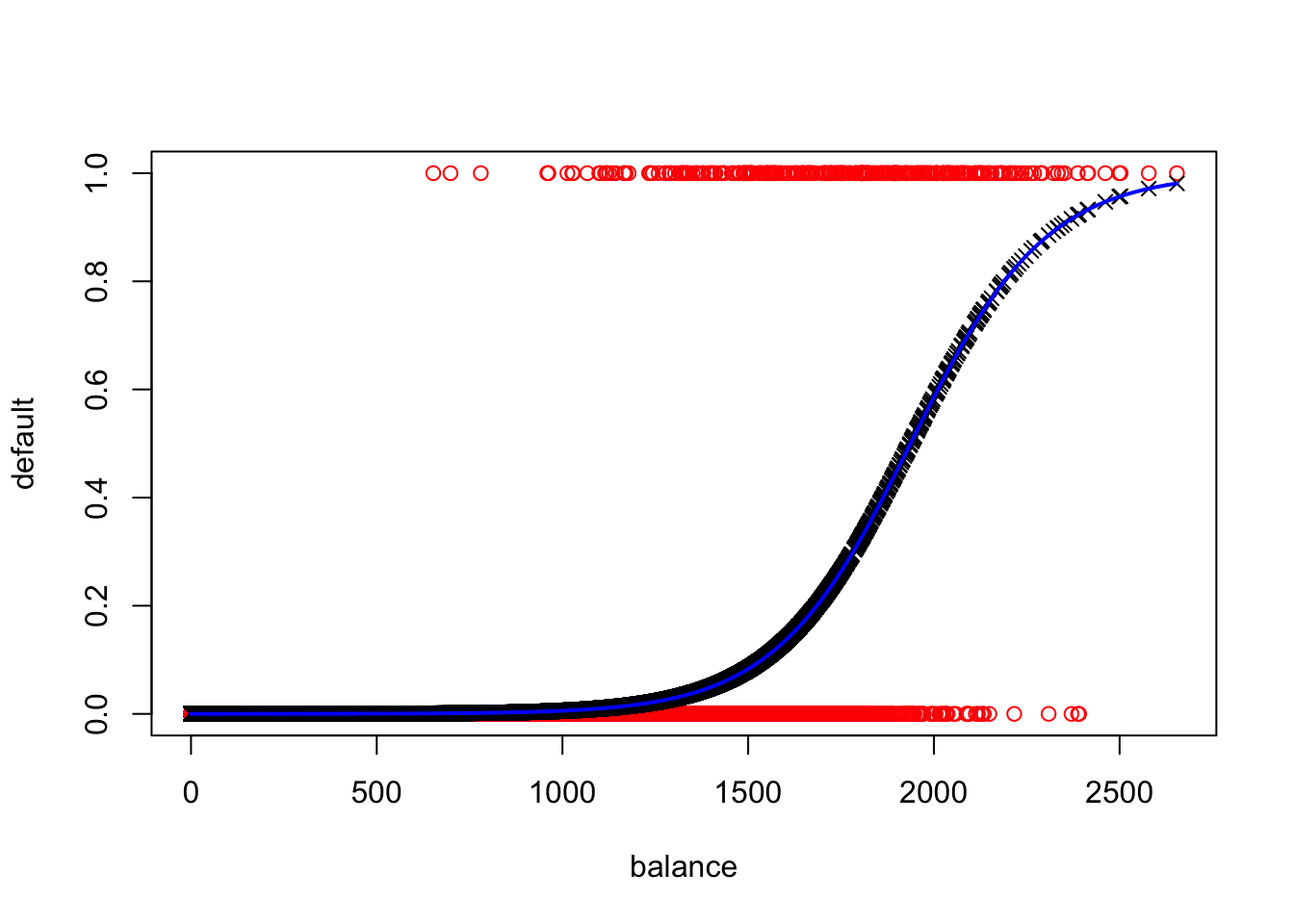

Predicting \(\hat{p}(X)\)

X = 1300
p.hat = exp(sum(glm.fit$coefficients*c(1,X)))/(1+exp(sum(glm.fit$coefficients*c(1,X))))
p.hat

## [1] 0.02923441

9.2 Multiple Logistic Regression

Pairs Plot (Factor Variable Coloured)

pairs(admit[,2:4], col=admit[,1]+2, pch=16)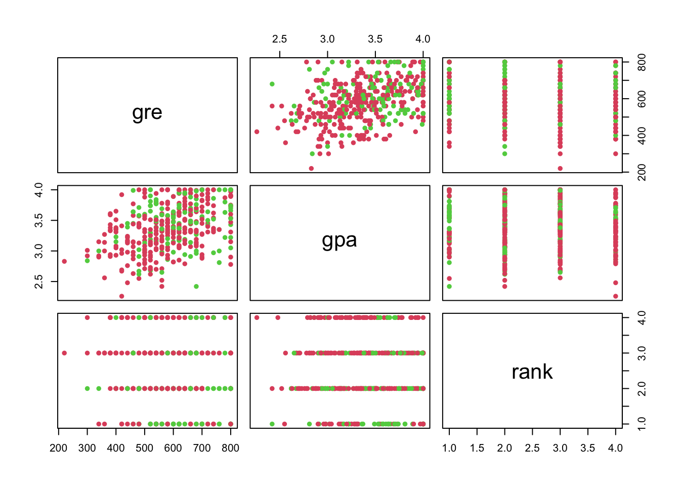

Making a Variable a Factor

admit$rank = factor(admit$rank)

Practical 4 Example

glm.fit = glm( admit ~ ., data = admit, family = "binomial")
summary(glm.fit)

## 
## Call:
## glm(formula = admit ~ ., family = "binomial", data = admit)
## 
## Deviance Residuals: 
##     Min       1Q   Median       3Q      Max  
## -1.6268  -0.8662  -0.6388   1.1490   2.0790  
## 
## Coefficients:
##              Estimate Std. Error z value Pr(>|z|)    
## (Intercept) -3.989979   1.139951  -3.500 0.000465 ***
## gre          0.002264   0.001094   2.070 0.038465 *  
## gpa          0.804038   0.331819   2.423 0.015388 *  
## rank2       -0.675443   0.316490  -2.134 0.032829 *  
## rank3       -1.340204   0.345306  -3.881 0.000104 ***
## rank4       -1.551464   0.417832  -3.713 0.000205 ***
## ---
## Signif. codes:  0 '***' 0.001 '**' 0.01 '*' 0.05 '.' 0.1 ' ' 1
## 
## (Dispersion parameter for binomial family taken to be 1)
## 
##     Null deviance: 499.98  on 399  degrees of freedom
## Residual deviance: 458.52  on 394  degrees of freedom
## AIC: 470.52
## 
## Number of Fisher Scoring iterations: 4

9.3 Inference

Calculating Probability

Use predict() function with type = "response" or type = "resp". The type = "response" option tells R to output probabilities of the form P(Y=1|X), as opposed to other information such as the logit. Do not include any data to calculate predictions for training data (used to plot the curve).

glm.probs = predict(glm.fit, type = "response")

Single Prediction/Multiple New Prediction

#Data For Prediction
testdata = data.frame(gre = 380, gpa = 3.61, rank = 3)
testdata$rank = factor(testdata$rank)

#Single Prediction
predict(glm.fit, testdata, type="resp")

##         1 
## 0.1726265

Predictions

Round probability to get a prediction.

#Prediction
glm.pred = round(glm.probs)

#Confusion Table
table(glm.pred, admit$admit)

##         
## glm.pred   0   1
##        0 254  97
##        1  19  30

#Ratio of correct predictions on test data
mean(glm.pred == admit$admit)

## [1] 0.71