Chapter 8 GAMs
We use the library(gam) package. Below is an example using the Boston data again.
library(gam)

names(Boston)
## [1] "crim" "zn" "indus" "chas" "nox" "rm" "age"
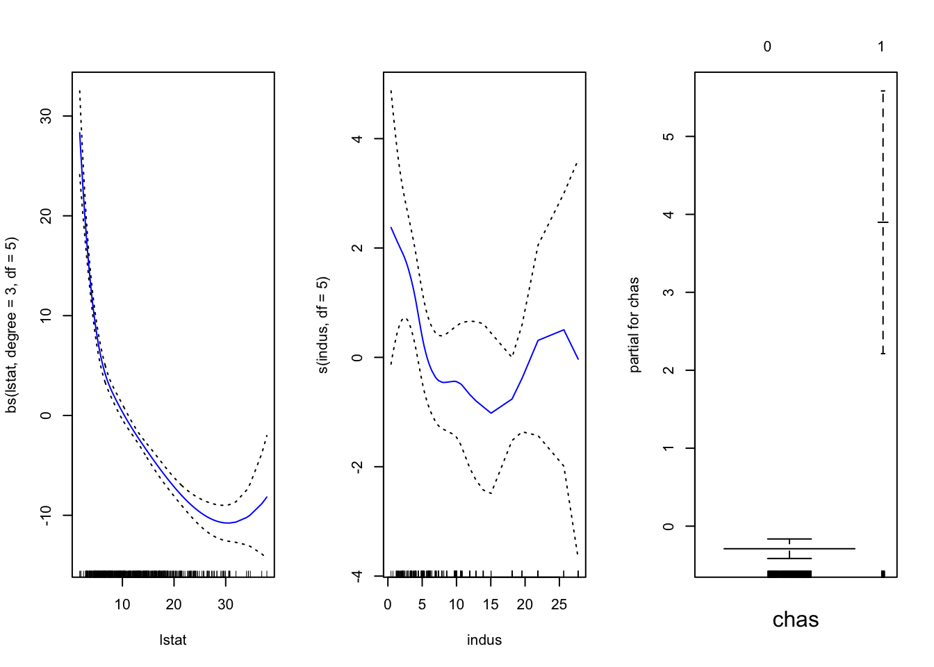
## [8] "dis" "rad" "tax" "ptratio" "black" "lstat" "medv"In this example we build a GAM using a cubic spline with 3 degrees of freedom for lstat, a smoothing spline with 3 degrees of freedom for indus and a simple linear model for variable chas. But first we make chas a categorical variable.
Boston1 = Boston
Boston1$chas = factor(Boston1$chas)
Practical 4 Example
library(faraway)
data("seatpos")

gam = gam(hipcenter ~ ns(Age, df = 5) + s(Thigh, df = 3) + Ht, data = seatpos)

par( mfrow = c(2,3) )
plot( gam,  se = TRUE, col = "blue" )
plot( seatpos$Age, seatpos$hipcenter, pch = 16, col = 2, ylab = y.lab, xlab = "Age (years)" )
plot( seatpos$Thigh, seatpos$hipcenter, pch = 16, col = 2, ylab = y.lab, xlab = "Thigh length (cm)" )
plot( seatpos$Ht, seatpos$hipcenter, pch = 16, col = 2, ylab = y.lab, xlab = "Ht (bare foot) (cm)" )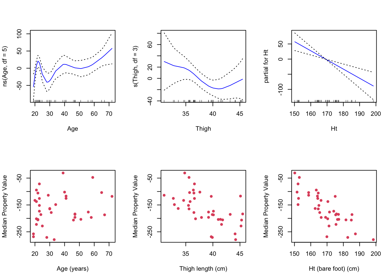
8.1 GAM Function
We use the gam() function which has the syntax gam( response ~ predictors + ..., data = data). The way to specify what the model of each predictor is is similar to lm().
bs()is used for a regression splinens()is used for natural spliness()is used for smoothing splines (this is different fromlmand how smoothing splines are done normally).
gam = gam( medv ~ bs(lstat, degree = 3, df = 5) + s(indus, df = 5) + chas, data = Boston1 )